|
Magnetic Flux Density
by
Robert L Rauck
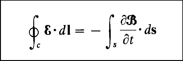
Faraday's Law states that the voltage induced in a single turn of wire wrapped around a magnetic core is equal to the rate of change of the magnetic flux enclosed by that wire. One of Maxwell's equations (generalizing Faraday's Law) asserts that the line integral of the Dot Product of the induced voltage vector and the differential path vector along a single turn of wire wrapped around a magnetic core equals the surface integral of the Dot Product of the rate of change of a magnetic flux density vector within that turn of wire and a differential surface integrated over the area enclosed by that wire. This version of the law is limited to stationary surfaces. This topic is sufficiently complicated to make many engineers look for an alternate career path.
This is, however, a very powerful assertion. If you know the rate of change of magnetic flux, you can compute the voltage that flux will induce in a wire that encircles it. The equation also allows you to predict the rate of change of flux in a core from the external voltage applied to a winding wrapped around that core.

|
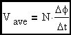
Solving the integral expression for the induced voltage in terms of the changing magnetic flux and generalizing to N turns. Note the minus sign that indicates that the induced voltage will oppose the applied voltage that is causing the flux change.
|
Let's now look at the expression involving the applied voltage that creates the changing magnetic field. The minus sign will be missing this time. Let's also make some simplifying assumptions that will be useful in evaluating practical magnetic devices.
|
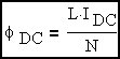
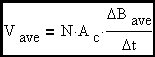
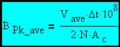
Faraday's Law with the voltage source replaced with an equivalent constant voltage set equal to the average value of the source (over the analysis interval). Note that ΔΦ is ΦP-P assuming that the voltage does not change polarity during the analysis interval
|
(Eq. 1)
|
|
&DeltaΦ = ΔBave•AC where ΔBave is the average value of BP-P for our purposes. We are dealing in MKS units initially. This expression assumes all the flux is confined to the core since we are using the core area. Average means averaged over the core cross-sectional area.
|
|
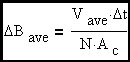
Simple rearrangement of terms
|
|
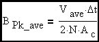
Substituting 2•BPK for BP-P and simplifying.
|
(Eq. 2)
|
|
Converting from MKS to CGS units since there are 104 Gauss / Tesla and 104 cm2 / m2 and 104•104 = 108. This is the general expression for the average value of peak flux density.
|
(Eq. 3)
|
Some general comments on the above equation are in order. The analysis computes the average value of peak flux density assuming that the flux is confined to the core. The errors in this assumption will be small only when the magnetic path is completely composed of very high permeability material and the device is operated to preclude core saturation. The addition of a core gap will lower the effective permeability of the path and degrade the accuracy of this analysis. As long as gap length is kept small relative to total path length, this effect will be minimized. Certain core types have an effective core cross-sectional area smaller than the actual core area due to construction from strips or stampings that are interleaved with nonmagnetic material. The equations should always use the effective core area found by multiplying actual area times the stacking factor. All practical magnetic cores, torroids for example, have a magnetic path length that varies over the cross-section of the core. These devices will exhibit peak flux densities that are highest where the path length is shortest (inside edge in the case of a torroid) and core saturation must be avoided for this worst case. Many core types also exhibit a cross-sectional area that varies along the path length. There are equations that have been developed to analyze the various core types and arrive at effective values for core parameters to use in magnetics design equations to account for geometric factors. If you are asking yourself how important this flux density gradient is; remember that if you have one foot in boiling water and the other foot frozen in a block of ice, on the average you are comfortable. This is one of the many reasons people do not design for the full flux density capability of the core. Others include temperature rise and the need for design reserve for cases where the circuit applies a transient to the magnetic device containing more than normal applied Volt•Seconds. Designs that have the possibility of DC current in the windings must be evaluated based on the peak flux due to all effects.
Now we will look at two common voltage waveforms (sinewave and squarewave) that arise frequently in magnetics analysis. We will assume, for simplicity, that there is no DC offset in the applied voltage for these cases. It will be noted that P-P flux swings (in opposite directions) will occur over each half-cycle of the applied voltage. The equations will focus on analysis over the positive half-cycle of the applied voltage in each case. We will drop the ave subscript in the following equations but it will be understood that we are always talking about average value of peak flux density.
|
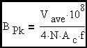
Taking the above CGS equation and substituting 1/(2•f) = Δt for the special case of a squarewave voltage.
|
(Eq. 4)
|
|
The equation for a squarewave does not change when Vrms is substituted for Vave since the RMS and Average values of a squarewave are the same (over a half-cycle of the waveform).
|
(Eq. 5)
|

|
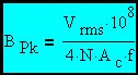
Taking Eq. 3 and substituting 1/(2•f) = Δt for the special case of a sinewave voltage. Result is same as squarewave (Eq. 4) as long as Vave is used!
|
(Eq 6)
|
|
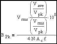
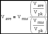
Taking Eq. 3 and substituting 1/(2•f) = Δt for the special case of a sinewave voltage where Vrms is used, requires a correction factorsince rms and ave are different for a sinewave (over a half-cycle of the waveform).
|
|
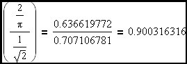
The correction factor times Vrms = Vave
|
|
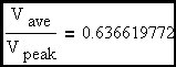
The ratio of Vrms / Vpk for a sine-wave is well known as 1/√2 and the ratio of Vave / Vpk will be derived below.
|
|
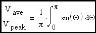
The average value of a sine-wave averaged over 1/2 cycle (0 to π radians) is the integral (area under the curve) divided by Δx which is π radians for a half cycle.
|
|
Evaluating the integral (step 1)
|

|
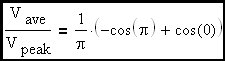
Evaluating the integral (step 2)
|
|
Evaluating the integral (step 3)
|
|
The final correction factor for the sinewave case.
|
|
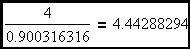
Combining this new correction factor with the 4 in the denominator of Equation 6.
|
|
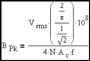
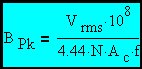
Final expression for the sine-wave case with voltage expressed as an RMS value.
|
(Eq 7)
|
We now can see why the equations for peak flux density in a magnetic device depend on the waveshape of the applied voltage. We also know, from the above discussion, that flux density varies over the core cross-sectional area and we are only looking at the average value with this analysis. Any design that applies a voltage waveform that can contain a DC component will also be subjected to a phenomenon known as flux-walking but that is a topic for another analysis.
The presence of DC current adds a bit of additional complexity.

|
This is the definition of inductance.
|
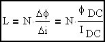
|
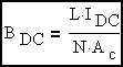
When inductance is constant over the current range of interest (MKS). There are certain specialized cases where this is not
the desired behavior but it holds for the vast majority of cases.
|
|
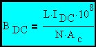
Converting from MKS to CGS since there are 104 Gauss / Tesla and 104 cm2 / m2 and 104 * 104 = 108.
|
(Eq 8)
|
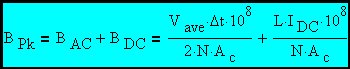
When an inductor is subjected to a DC current and an AC voltage, the total peak flux density is the sum of two components (Eq. 3 & Eq. 8).
|
|
(Eq 9)
|
The previously developed expressions for special voltage waveshapes can be substituted for the voltage dependent term in Eq. 9.
|